The part looked simple: a small bracket with straightforward geometry and a clear function.

But when final assembly began, the issue appeared.
Tool access was tighter than expected, installation space was limited, and the mounting sequence became less convenient than it seemed in the model.

Nothing was dramatically wrong with the part itself.
The challenge came from how the part behaved in the real assembly environment.

This is a common reminder in sheet metal development:
a part can look simple in CAD and still become a bottleneck at the final stage.

#SheetMetal# #Assembly# #MechanicalDesign# #Manufacturing# #BracketDesign# #ProductDevelopment

Many cost increases do not come from the overall part size.

They come from specific details.

Sometimes it’s:

• an unnecessarily tight tolerance
• a difficult feature position
• too many secondary operations
• a finish requirement added late
• complex hardware insertion needs
• packaging or protection requirements that were overlooked

These things may seem minor at first, but they can significantly affect manufacturing cost and lead time.

What part detail has caused the biggest unexpected cost increase in your experience?

This could be a useful discussion for engineers trying to design more cost-aware parts from the start.

#SheetMetal ##CostOptimization# #Manufacturing# #Engineering# #DesignForCost# #HardwareDesign# #Production#

In some sheet metal projects, the best structural choice is not always the best visual choice.

For example:

• a stronger feature may affect external appearance
• a more practical bend may change the product style
• visible fasteners may be easier to assemble
• a cleaner surface may require more process control

This balance shows up often in enclosures, consumer-facing hardware, and branded equipment.

So here's the question:

When appearance and function conflict in a sheet metal part, which one usually wins in your project — and why?

It would be great to hear how different teams make that decision.

#sheetmetal# #surfacefinish#

Surface finishing is often treated as a default step—but in some cases, it can actually cause more problems than it solves.

Here are situations where skipping finishing might be the better choice:

🔹 Tight Tolerance Assemblies

Coatings like powder coating or anodizing add thickness.

Even a small buildup can affect fit, alignment, or clearance.

👉 Raw parts may ensure better precision in critical fits

🔹 Electrical Contact Surfaces

Some finishes (like standard anodizing) reduce conductivity.

👉 For grounding or electrical interfaces, raw metal or conductive finishes are often preferred

🔹 Cost-Sensitive Prototypes

Surface finishing adds both cost and lead time.

👉 For early-stage testing, raw parts are often enough

🔹 Hidden/Internal Components

If the part isn't visible or exposed to harsh environments, finishing may not add real value

🔹 Post-Processing Required

If parts need additional machining, tapping, or welding after fabrication:

• Coating may get damaged
• Extra steps may be needed

💬Discussion:

Have you ever skipped surface finishing intentionally?

What was your deciding factor—cost, function, or assembly?

#sheetmetal#

#surfacefinish#

Surface finishing isn't just about appearance—it affects durability, conductivity, corrosion resistance, and even assembly fit.

Here's a quick breakdown of common sheet metal finishes:

🔹 No Finish (Raw)

• Lowest cost, fastest turnaround
• Keeps original material properties
• May oxidize or scratch easily

👉 Best for internal parts or quick prototypes

🔹 Brushing

• Creates a uniform, textured surface
• Improves visual consistency
• Does not provide strong corrosion protection

👉 Often used for aesthetic aluminum or stainless parts

🔹 Powder Coating

• Thick protective layer
• Excellent corrosion resistance
• Wide range of colors
• Adds thickness (important for tight fits)

👉 Great for enclosures and outdoor applications

🔹 Anodizing (Aluminum)

• Improves corrosion resistance
• Creates clean, premium look
• Maintains relatively tight tolerances

👉 Common for consumer-facing aluminum parts

🔹 Hardcoat Anodizing

• Much thicker and harder than standard anodizing
• High wear resistance
• Slight dimensional change

👉 Used in high-friction or industrial environments

🔹 Conductive Anodizing

• Maintains electrical conductivity
• Provides light corrosion protection

👉 Ideal for electronic housings and grounding applications

🔹 Silkscreen

• Used for logos, labels, markings
• Typically applied after coating or anodizing

👉 Great for branding and instructions

🔹 Laser Marking

• Permanent, high-precision marking
• No added thickness
• Very durable

👉 Used for serial numbers, QR codes, branding

💬 Discussion:

When choosing surface finishes, what matters most in your projects—appearance, durability, or functionality?
Have you ever had issues with coating thickness or finish affecting assembly?

#sheetmetal# #surfacefinish#

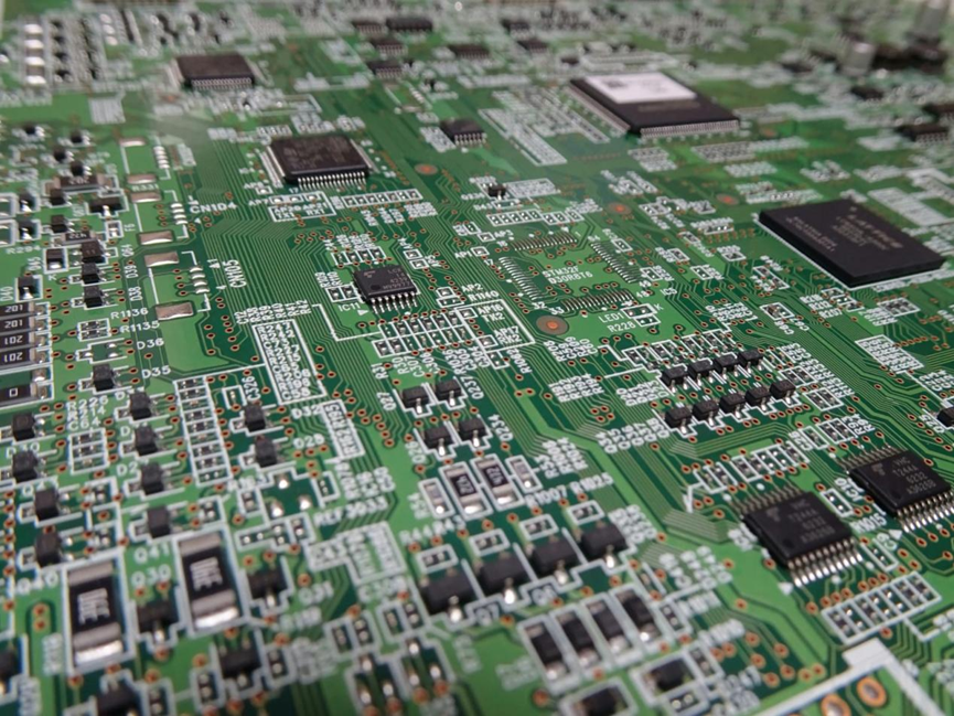
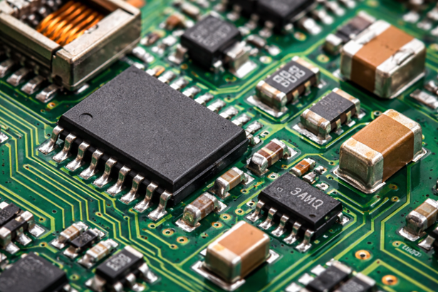
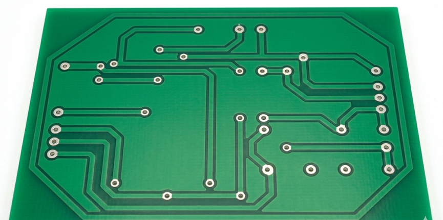
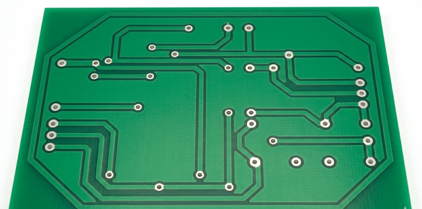
PCB trace close-up (conceptualized)

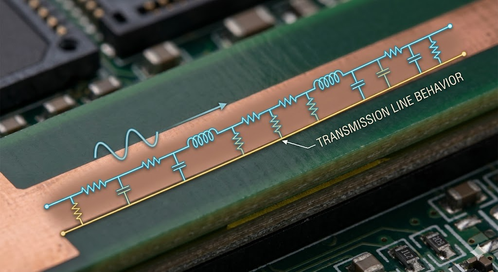
Signals, in PCB design, are not instantaneously transmitted, but rather propagate as electromagnetic waves over copper traces, which is fundamental to understanding why trace-length can be critical to signal integrity.

The speed at which a signal propagates depends on the material in which the signal is propagating, with typical standards for FR-4 PCB materials being approximately 50-70% of the speed of light. Thus, a signal propagating from one PCB pad to another may take 100 + picoseconds to travel a nominal distance of 2-3 centimeters. This travel time is relatively significant when compared with the fast rising (edge rate) of the signal itself.

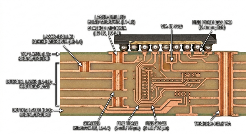
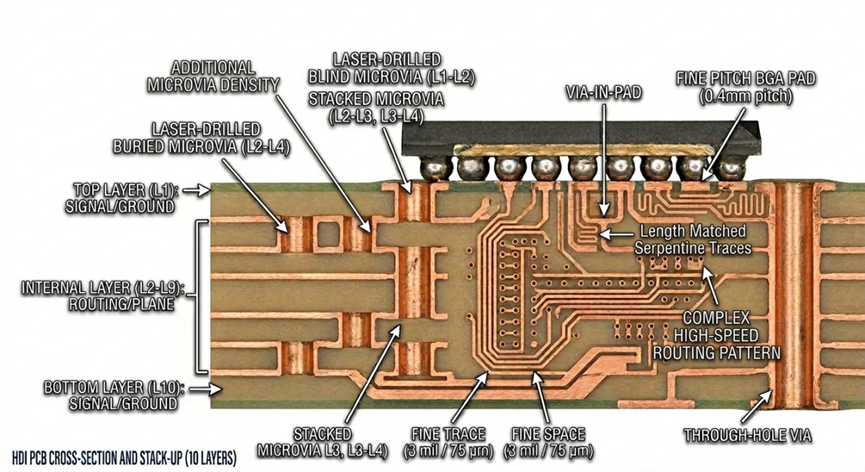
High-density PCB routing

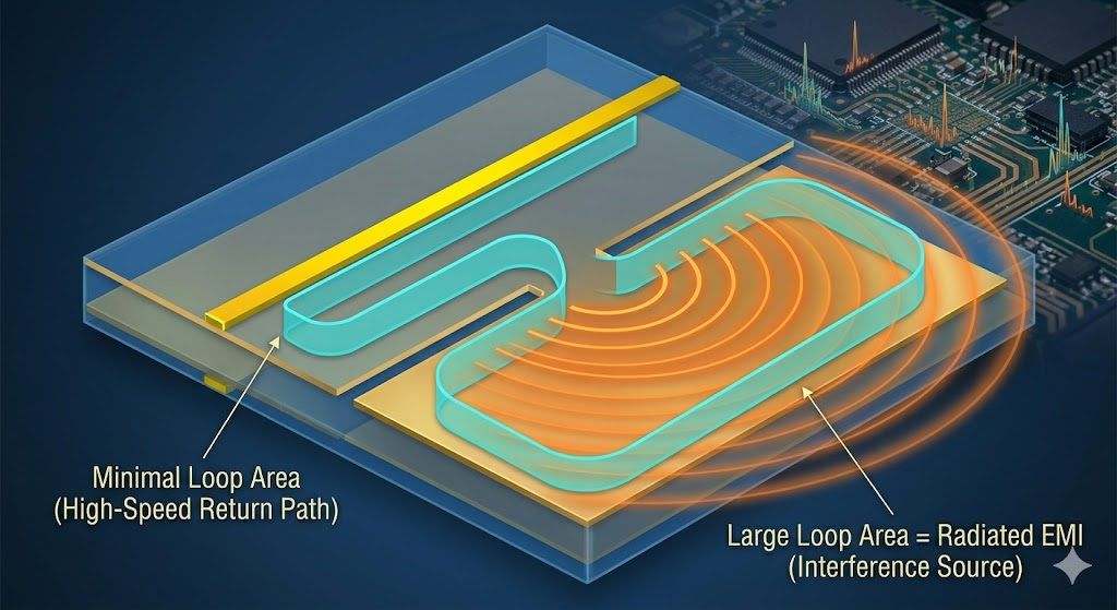
In addition to the delay of a signal traveling on its forward path, the signals also have a return path back to the source, typically by way of a common ground. Increased trace lengths create larger return loops, therefore increasing the inductance and the effects of voltage/potential noise from any external electromagnetic interference (EMI) sources.

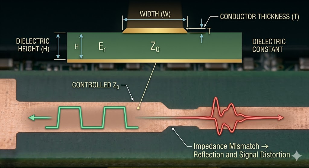
Higher trace lengths increase resistive/capacitive characteristics, which in turn may attenuate the signal, create longer rising/falling signals, and create potential distortion. When considered at higher frequencies, traces can behave like transmission lines, where impedance mismatching effects create reflections. Reflections can introduce ringing, as well as logic errors.

Timing is another major consideration. When considering buses or high-speed interfaces, a difference in trace length will cause some skew (i.e., signal arriving at different times). This will potentially cause the system to lose its intended relationship of synchronization for such devices as memory or differentials.

The reason designers apply techniques such as length matching, controlled impedance routing, and appropriate terminations is because keeping traces as short, direct, and grounded to the reference plane will help to maintain the integrity of the signal.

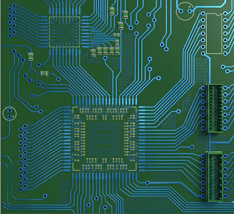
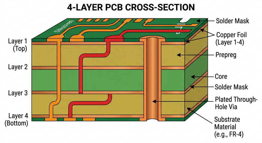
PCB with short, direct, and grounded traces

Takeaway? Trace length is not simply an attribute of geometry; it impacts the manner in which the signal behaves. As speeds continue to increase, propagation management is critical to reliable and predictable circuit operation.

When designing printed circuit boards (PCBs), "high speed" is not solely determined by clock frequency, but rather by the rate at which signals are switching (rise and fall times). When rise/fall times are down to the point where they are close to the speed it takes to propagate a signal along a trace, layout becomes very important; as a rule of thumb, when the length of a trace exceeds approximately 1/10th of its effective wavelength (also called edge length), it must be treated as if it were a transmission line. At that point, reflection, impedance mismatch, and ringing will create distorted signals.

PCB close-up

This is why "slow" systems (e.g., tens of MHz) may require fast design techniques if they incorporate very fast digital logic families with very sharp edges.

Three layout considerations are particularly important for high-speed circuit designs; controlled impedance (all traces and cables have impedance), continuous ground plane (a common reference with low impedance), and tightly coupled return path (the return current flow follows the path of least impedance; in most cases directly under the trace). In high-speed applications, signals form loops, and return current finds the path of least impedance, typically directly under the trace. Interruptions (such as ground splits) will increase the total area of the loop and increase the amount of electromagnetic interference (EMI).

Dense PCB routing / high-speed layout

When designing for fast applications, crosstalk must also be taken into account. Two close traces that run parallel and adjacent to each other can couple energy to one another over long cable lengths. Proper trace spacing and layer management will help reduce the amount of crosstalk present in a design.

PCB layer management can be an important factor to consider

Interface Standards are another triggering mechanism. Controlled routing (i.e., differential routing methods) and matched lengths are required of signal traces regardless of clock rate for Protocols such as USB, Ethernet and DDR memory.

The takeaway from this is that the phrase "High Speed" is defined as beginning at the point where physics (not simply connectivity) starts to govern signal behavior. Therefore, if you have fast edge rates, long trace lengths, or tight timing constraints on your signals, layout is critical for successful operation.

E-Ink Display

E-Ink displays are an excellent choice for low-energy IoT dashboard systems because they only draw power when being updated. Unlike LCD screens which require a constant supply of power to maintain an image, E-Ink displays retain an image without needing any power applied. Therefore, they are a great fit for battery operated systems that require data to be updated from time to time.

This characteristic makes E-Ink displays well-suited for applications such as sensors, status information, and remote monitoring devices that don't update often. When combined with low power microcontrollers, E-Ink displays can endure for months or years with small batteries.

E-Ink displays have lower refresh rates and only have limited colors. So, they are best for displaying static or slowly changing data.

The end result is ultra-low power visualisation while retaining readability, even in bright conditions.

There are several benefits when integrating MQTT with Python for real time data visualisations. MQTT has been specifically designed for low-bandwidth devices as a light-weight publishing/subscriber protocol. To create a real-time visualisation of IoT devices using the Python programming language, paho-mqtt is a library that can be used to subscribe to sensor devices and stream in real time the data from those sensor devices into visualisation tools such as Matplotlib and Plotly.

The way this workflow works is you connect to an MQTT broker, subscribe to the relevant sensor device topics, and when the broker receives an update it sends an update to the subscribers (your Python script) which in turn automatically updates the visualisation of the data points using either Matplotlib or Plotly.

MQTT (Message Queuing Telemetry Transport)

Therefore, with an integrated form of Python and MQTT, users are able to create an easily accessible Dashboard that displays live data which is much easier to monitor and debug.

TLS (Transport Layer Security) is used to secure IoT devices through encrypted communications. In this case embedded hardware must use light weight libraries and have a proper way to manage recourses.Use the same secure key storage methods and secure elements (e.g., ATECC608A) to ensure that you cannot extract your private keys.

Ensure you are using the latest cipher suites (e.g., AES, ECC), and that you have a complete certificate validation process to help prevent MITMs. Handshakes in TLS require a large amount of resources therefore re-use sessions where possible and reduce the number of reconnections may help to save resources.

The purpose is not just encryption but also authentication and integrity of the device only communicating with authenticated servers.

The Critical Role of Ground Planes in High-Speed PCB Design: When developing a printed circuit board, the implementation of a solid ground plane is far more than a structural choice; it is a fundamental requirement for signal integrity.

Why Continuity Matters: In high-frequency systems, signals propagate as electromagnetic waves within a transmission line environment. A continuous copper plane directly beneath the signal trace provides a predictable, low-inductance return path. If this plane is fractured or interrupted, the return current cannot follow its ideal path. Instead, it is forced to "detour" around the gap. This deviation increases the loop area of the circuit, causing the electromagnetic fields to expand and bleed into neighboring traces. This mechanism is the primary driver of crosstalk and electromagnetic interference (EMI).

Empirical Evidence: A Comparative Study To quantify the impact of ground plane integrity, we can examine a laboratory setup involving two distinct PCB configurations. Both boards utilize matched 50Ω striplines, each terminated into a 50Ω load to the underlying ground plane. Each board features two connectors, labeled H1 and H2. The Experiment: A high-speed signal is injected into H1 (the "aggressor" line), while the signal on H2 (the "victim" line) is monitored on two different PCBs. The first one (PCB4) has an interrupting trace under both H1 and H2 while the second one has an interrupting trace only under H1 (PCB3). To do the experiment, two waveforms have been injected, a square wave and a sine wave both at 5V, and the peak-to-peak crosstalk voltage and its dependency on frequency have been found. Then, applying different frequencies, different data have been acquired.

Data analysis: From the data it is possible to notice how crosstalk is significantly higher for the PCB4 in both settings: square and sine waves applied. Also, with higher frequencies come also higher crosstalk.

Conclusion: When designing a PCB's layout, guaranteeing that one of the ground planes is solid without any cutting is actually very significant and can guarantee a good output of the PCB reducing crosstalk and thus disturbs.

#PCB##PCB# #PCB# #layout# #grounding# #loop# #current# #PCBDesign#

#decoupling# #capacitor# #pcb design# #JLCPCB#

Lately I have had this doubt: is the position of the decoupling capacitor really significant? Well, the quick answer is YES!

Here you will see a brief experiment and its results that I hope will make you understand how significant actually is.

First of all, what are decoupling capacitors and why are they needed?

• Well, they are needed to stabilize voltage and eliminate noise in electronic circuits by providing a local and high-speed reservoir for components (such as microcontrollers etc.). It will prevent the EMI radiation, as well as isolate the sensitive components from the power supply noise. More specifically, when a circuit needs current instantly the supply rails can't react instantly because of wiring inductance and resistance, thus the supply voltage sags. Putting a decoupling capacitor helps with this by keeping the circuits stable.

What do you need? 

• An oscilloscope, a signal generator and a power supply. The circuit built featured a NPN BJT transistor, with a resistor of 20 Ohm on its source, the gate connected to ground and drain to Vcc. Connected to the gate there was a source generator generating a square wave of 5V of amplitude at 1kHz. The source was connected to the scope/oscilloscope with DC coupling.
• After building the circuit with a breadboard, you can put a capacitor at difference distances from the voltage source and see its effect on the voltage drop.

Obtained data analysis

• the voltage drop without a capacitor is around 4.62V. This is HUGE! Since the voltage power is of 5V.
• the 1000uF electrolytic/ 1uF film capacitors are the one that reduced more significantly the voltage drop. Generally the electrolytic however are slower.
• the more the capacitor is near to the voltage source the more it attenuates its voltage drop.

Key findings from data

The experimental data reveals a critical struggle between power stability and signal speed. Without any decoupling, the 4.62V drop on a 5V rail represents a near-total power failure every time the transistor switches. In a real-world application, this wouldn't just be electrical noise; it would cause a processor to brown out or a sensor to provide false readings because the voltage hits rock bottom.

These results also expose a performance trade-off tied to internal resistance. The 1000uF electrolytic capacitor acts like a massive water tank with a slow, narrow valve. While it holds enough energy to prevent the voltage from sagging, it cannot release that energy fast enough to keep up with the 1kHz square wave. This explains why the signal rise time slowed to 153ns with the large cap, whereas the 1uF film version, acting as a smaller but much faster bucket, snapped the signal into place in just 90ns.

CONCLUSION

When designing a PCB's layout, ALWAYS put the decoupling capacitors near its voltage source, the nearest the better!

Do not put them distant!!

The Inverted-F Antenna (IFA) is an ideal option for 2.4GHz applications (Wi-Fi, Bluetooth) as it is small in size and performs well on basic 2 layer PCBs.

PIFA

An IFA acts like a quarter wavelength radiator. For 2.4 GHz the wavelength is approximately 125 mm so the actual radiating length will be 25 - 30 mm tall on FR-4 as a result of the dielectric material. However, because the antenna is housed on a PCB (which introduces dielectric loading), actual IFA length will typically range from 20-30mm in FR-4 material.

Three components make up the structure of an IFA:

1. Radiating Element/Main Trace
2. Shorting Pin/Trace To Ground
3. Feed Point Located Between The Other Two Components

The shorting component reduces the resonant length of the radiator and aids in impedance matching, while the feed location will allow for further fine-tuning of input impedance (targeted value of approximately 50Ω).

Proper ground plane design is also essential. The IFA should ideally be placed at the edge of the PCB with no copper and no routing underneath and around it (the keep-out area). The remaining area of the PCB acts as the ground plane; thus, the size and shape of the ground plane will have a large influence on performance.

Dedicate the entire bottom layer of a PCB with 2-layers as a solid ground plane and use multiple vias near both the feed and shorting locations to ensure a low-impedance path to ground.

Tuning is a necessary step that cannot be avoided. A small change in an object's length or width, or objects around the object, will affect the resonance. By including a π-matching network in the feed using two capacitors and one inductor, you can fine-tune your fabrication using a VNA after fabrication.

VNA

So what have we learned? Antenna design is split equally between calculation, layout discipline and tuning. Once you have your geometry and grounding right, you end up with an efficient, reliable antenna without having to rely upon elaborate multilayer boards.

PCB close-up

High-frequency circuit board design (microwave design) applies not only to radio frequency circuit board design engineers, but also to today's designers of circuit boards. Circuit board, or PCB, designers use microwave design principles as they reach frequencies of hundreds of MHz or more, where traces on Printed Circuit Boards (PCBs) are no longer behaving as simple wire connections, but will instead function as transmission lines.

Controlled impedance is an important concept in PCB design. Each PCB trace has a characteristic impedance that is determined by the construction parameters of that trace: Width, thickness of conductor materials, dielectric materials used as well as the distance to the reference or ground plane. Impedance mismatches (discrepancies between the characteristic impedances) create reflections/echoes and signal integrity issues in the form of signal loss and/or distortion. As a result controlled PCB geometric shapes must be closely adhered to; otherwise, you will create a signal integrity and performance issue.

Another important concept is return path. High frequency signals will follow the path of least impedance, which will normally be directly underneath the PCB trace (on the ground plane). Any type of discontinuity (for example, split planes) will increase the loop area and cause interference problems in the forms of radiated Electro Magnetic Interference (EMI).

Material selection is important too; standard FR-4 laminate will work on many PCB applications, but as you increase frequency you have increased dielectric losses. Therefore, in high frequency applications (i.e greater than 1GHz), it is common to select lower-loss laminates to maintain signal integrity.

In addition to using proper design parameters & materials, PCB layout techniques will change when designing high frequency PCBs. Design Engineers must consider design matching of trace lengths, effects of vias (splices in traces), and parasitic types of effects. Little elements within a PCB like stubs and sharp bends can have performance ramifications. Therefore, proper routing can be vital to achieving good signal integrity.

In conclusion, the use of simulation tools and measurement tools such as field solvers and vector network analyzers (VNA’s) are an important part of validating both pre-production and post-production designs.

The bottom line for microwave PCB designs is to help control the flow of energy through the circuit as opposed to simply connecting all points. By mastering these basic components of circuit design, you will now be able to produce circuits that function reliably and with superior performance at increasingly higher frequencies.

Three factors will aid you in your determination of which network is best for your IoT application: Coverage, power, and infrastructure.

LoRaWAN is the best candidate if your IoT application requires a network to work out of the grid, or in rural areas. LoRaWAN operates in an unlicensed band, has a long range (up to several kilometres), and consumes very little power – requiring batteries to last for multiple years.In addition, you can use private gateways for your device to provide access to the internet.

NB-IoT (Narrowband Internet of Things) is a licensed cellular technology that has been approved by 3GPP and utilizes existing LTE networks and licensed spectrum. With NB-IoT as an option, you have another viable method of connecting your devices to the Internet; how to do this depends on your needs. NB-IoT also has very good Quality of Service (QoS) because of its direct connection to either the Internet/cloud. While NB-IoT provides a reliable connection for several devices connected to the Internet, it can draw considerably more power than LoRaWAN and is therefore subject to some restrictions on carrier network connectivity.

Side by side LoRa module and NB-IOT module

Your best option for flexibility and extra low power consumption would be the LoRaWAN option, though if you need a mobile/cellular carrier level of reliable connectivity (with[during and after] supported network issues), then you would want to use NB-IoT instead.

To achieve 2-year battery life from one LiPo cell, you must practice aggressive power management. Start with a low consumption MCU and utilize deep sleep modes whenever possible, as many of the more modern MCUs will draw microamperes (µA) when idle. Use duty-cycling for everything, including the sensors, the radios, and even the regulators; they should turn on only when needed.

You can reduce the transmission time in all wireless communications (LoRa, WI-FI, BLE); wireless communications typically consume the largest amount of power. Make sure your firmware has been revised to allow for the controllers to be in sleep mode for an extended period of time in order to allow for quickly waking up, collecting data, transmitting data and returning to sleep mode. Additionally, reduce the quiescent current from your regulators and periphery.

The key to longevity is not purchasing a much larger battery; it is how much time the device spends in sleep mode.

The ESP32 is superior in the aspect of connectivity, with built-in Bluetooth and wi-fi. It is an exceptional device to use as a gateway for collecting, forwarding and transmitting information without having to use additional hardware. Additionally, the ESP32 has a large ecosystem, allowing for quick models to be deployed.

On the other hand, STM32 microcontrollers focus on reliability, low power, and deterministic performance; normally, they require additional RF Modules (LoRa, Sub-GHz). Depending on the use case, it will give greater real-time control to the gateway and industrial-grade reliability.

In conclusion, the ESP32 is an effective solution for fast, connected gateways, while the STM32 is an effective solution for a complete, robust, long-range unified solution by combining the best of both microcontrollers for efficient long-term operations.

Making clean Gerber files is the final stage between your design and a successful build. While there are different workflows with the use of the different tools used for generating Gerber files, the main fundamentals are always consistent - specifically for preparing files for JLCPCB.

First, go to KiCad. Then, Use the Plot menu. Typically, various layers must be output from the Plot menu in RS-274X format. You will not have a drill layer combined with your other layers when making the Gerber files. It’s extremely important that you process your drill layer independently of your other layers.

Once the Gerber files have been generated, you should also check the Gerber files for plotting accuracy using the internal viewer.

Gerber file preview / PCB layers visualization

In EAGLE, using a CAM Processor will allow users to load in a standard job Gerber file and generate all required layers. Be sure to double-check names when renaming layers to avoid any confusion.

Though EasyEDA does not create GERBERS by hand, users must still review output layers and preview before submitting order.

Gerber file preview / PCB layers visualization close-up

If using OrCAD, you will need to use the Manufacture → Artwork process. You will define the film output for the layers you require, as well as when you export to the NC drill files.

Regardless of the software you are using, there are three main steps that you will always need to do in order to prepare your final output – always include all of the layers required, always know what units you are using, and always verify the generated output prior to submitting it. A quick verification in a Gerber viewer may help prevent an expensive mistake in fabrication.

PCB with a green solder mask coating applied

PCBA shortages occur - good design planning can keep you moving forward. First, look for drop-in replacement parts - these should have the same packaging, pinout, and electrical specifications. If that's not possible, find functionally equivalent parts so that you can modify the design as early as possible. Use platforms like JLCPCB to see real-time availability of the component during your bill of materials (BOM) generation process.

Datasheet comparison is critical. If you want to avoid having to redesign your entire system at a later date simply because certain components are no longer available through the supply chain, putting enough design flexibility into your design early on will allow you to do so without any major inconvenience. Voltage tolerances, timing requirements, voltage ranges, and footprints must all be the same as specified in your specifications for the components used in your system.

The most important factors for any industrial air quality monitor are its accuracy and reproducibility. So I typically use JLCPCB since they combine PCB fabrication, SMT assembly and parts sourcing into one workflow to avoid handling errors and to maintain consistent builds across different batches.

For sensor-based designs, assembly quality has to be stable. Proper soldering, precise placement, and controlled process variables all contribute to retaining calibration and consistent performance over time. The availability of a large selection of components also makes it easier to source sensors, MCUs, and power components.

When combined with fast delivery times, this results in efficient iterations of products so they can be tested, adjusted and put into production.

Layout view of my PCB

Engineering a Robust Ecosystem

The heart of this system is the ESP32-WROOM-32U, providing the computational power and connectivity needed for real-time edge processing. By choosing JLCPCB, the transition from this complex, multi-layer design to a physical board was flawless, ensuring signal integrity for the high-sensitivity sensors integrated into the array.

Multi-Sensor Integration

To provide a comprehensive overview of environmental health, the board features a curated selection of industrial-grade sensors:

• MQ136 Gas Sensor: Specifically chosen for targeted gas detection (such as Hydrogen Sulfide), broadening the monitor's utility in specialized industrial zones.
• CCS811: For monitoring Total Volatile Organic Compounds (TVOCs) and equivalent CO2 levels.
• DFRobot SHT31-D: A high-precision digital temperature and humidity sensor protected by a PTFE membrane for long-term stability.

Power Management for the Field

Reliability in the field depends on power stability. The design incorporates a sophisticated power path:

• TP4056 Charging Module: Manages the 3.7V Li-ion battery lifecycle via USB.
• LM2596 Buck Converter: Ensures an efficient step-down to 3.3V/5V rails, maintaining steady operation even as battery levels fluctuate.